Databases rely on indexes to quickly locate and retrieve data that is stored on disks. While traditional database indexes use tree data structures such as B+ Trees to find the position of a given query key in the index, a learned index structure considers this problem as a prediction task and uses a machine learning model to “predict” the position of the query key.
Traditional and learned indexes | ML models to approximate the CDF |
---|---|
This novel approach of implementing database indexes has inspired a surge of recent research aimed at studying the effectiveness of learned index structures. However, while the main advantage of learned index structures is their ability to adjust to the data via their underlying ML model, this also carries the risk of exploitation by a malicious adversary.
This post will show some experiments that I have conducted as a follow-up to the research on adversarial machine learning in the context of learned index structures that was part of my master’s thesis at The University of Melbourne.
In my master’s thesis, I have executed a large-scale poisoning attack on dynamic learned index structures based on the CDF poisoning attack proposed by Kornaropoulos et al. The poisoning attack targets linear regression models and works by manipulating the cumulative distribution function (CDF) on which the model is trained. The attack deteriorates the fit of the underlying ML model by injecting a set of poisoning keys into the dataset, which leads to an increase in the prediction error of the model and thus deteriorates the overall performance of the learned index structure. The source code for the poisoning attack is available on GitHub.
As part of the experiments for my master’s thesis, I evaluated three index implementations by measuring their throughput in million operations per second. The evaluated indexes consist of two learned index structures ALEX and Dynamic-PGM as well as a traditional B+ Tree. Because indexes are usually used to speed-up data retrieval when dealing with massive amount of data, I chose to evaluate the performance of the indexes based on the SOSD benchmark datasets that consist of 200 million keys each.
Unfortunately, executing the poisoning attack by Kornaropoulos et al. is heavily computationally intensive, so I had to run them with a fixed poisoning threshold of $p=0.0001$, thus generating 20,000 poisoning keys for a dataset of 200 million keys. This poisoning threshold can be considered to be relatively low, as previous work on poisoning attacks has used poisoning thresholds of up-to $p=0.20$.
To test the robustness of learned indexes more rigorously, I have set-up a flexible microbenchmark that can be used to quickly evaluate the robustness of different index implementations against poisoning attacks. The microbenchmark is based on the source code that was published by Eppert et al. which I have extended to implement the CDF poisoning attack against different types of regression models and the learned index implementations ALEX and PGM-Index.
The corresponding source code can be found here: https://github.com/Bachfischer/LogarithmicErrorRegression.
To test the robustness of the learned indexes, I have generated a synthetic dataset of 1000 keys and ran the poisoning attack against each index implementation while varying the poisoning threshold from $p=0.01$ to $p=0.20$.
The graphs below show the performance deterioration calculated as the ratio between the mean lookup time in nanoseconds for the poisoned datasets and the legitimate (non-poisoned) dataset.
SLR | LogTE | DLogTE | 2P |
---|---|---|---|
TheilSen | LAD | ALEX | PGM |
---|---|---|---|
From the graphs, we can observe that simple linear regression (SLR) is particularly prone to the poisoning attack, as this regression model shows a steep increase in the mean lookup time when evaluated on the poisoned data.
The performance of the competitors that optimize a different error function such as LogTE, DLogTE and 2P (introduced in A Tailored Regression for Learned Indexes) are more robust against adversarial attacks. For these regression models, the mean lookup time remains relatively stable even when the poisoning threshold is increased substantially.
Because SLR is the de-facto standard in learned index structures and used internally by the ALEX and the PGM-Index implementations, we would expect that these two models also exhibit a relatively high performance deterioration when evaluated on the poisoned dataset. Surprisingly, ALEX does not show any significant performance impact, most likely due to the usage of gapped arrays that allow the model to easily capture outliers in the data (this effect can be likely attributed to the small keyset size). The performance of the PGM-Index deteriorates by a factor of up-to 1.3x.
To put things into a broader perspective, I have also calculated the overall mean lookup time for the evaluated learned indexes (averaged across all experiments) in the graph below.
We can see that ALEX dominates all learned index structures. The performance of the regression models SLR, LogTE, DLogTE, 2P, TheilSen and LAD is also relatively similar, in a range between 30 - 40 nanoseconds.
In the experiments, PGM-Index performs worst with a mean lookup time of > 50 nanoseconds. This is most likely due to the fact that PGM-Index is optimized for large-scale data workloads and exhibits subpar performance in this microbenchmark because the dataset consists of only 1000 keys.
I consider the results from this research to be a highly interesting study of the robustness of learned index structures. The poisoning attack and microbenchmark described in this post are open-source and can be easily adapted for future research purposes. If you have any further thoughts or ideas, please let me know!
]]>The task of the project was to develop a method to estimate the coordinates from which an image was taken. The dataset for this task was published by the COMP90086 teaching team and consisted of a collection of images taken in and around an art museum (the Getty Center in Los Angeles, U.S.A.).
The training dataset contained a total of 7500 images labeled with their corresponding (x,y) coordinates. The test dataset for which the coordinates should be predicted contained 1200 images.
For our participation, we chose to use the pre-trained SuperGlue model to extract features from the images in the training set and match them with the images in the test set.
The image above shows the SuperGlue network architecture and is taken from the original SuperGlue paper by Sarlin et al. SuperGlue combines a graph neural network architecture and attention mechanism to match local image features by finding correspondences and dismissing unmatchable points. It consist of two main components:
In the first component (Attentional Graph Neural Network), SuperGlue borrows the self-attention mechanism from Transformer and embeds it into a Graph Neural Network. The attentional GNN leverages spatial relationships of keypoints and descriptors. It works by first employing an encoder to map keypoint positions $p$ and their associated descriptors $d$ into a single vector. In the next step, self-attention and cross-attention layers are used to generate more powerful representations $f$. This component consist of a total of 9 layers of self- and cross-attention with 4 heads each.
The second component (Optimal Matching Layer) creates an $M \times N$ score matrix and finds the optimal partial assignment between two sets of local features by using the Sinkhorn algorithm for $T = 100$ iterations.
The pre-trained SuperGlue model consisting of approx. 12M parameters has been implemented in PyTorch and available on GitHub. It can be amalgamated with any local feature detector and descriptor techniques such as SIFT and SuperPoint to extract sparse keypoints and perform matching. In our experiments, SuperGlue was able to estimate almost all correct matches while rejecting the majority of outliers.
Shown below is an example from the COMP90086 dataset. An example image from the test set is shown on the left, and the corresponding image from the training set is shown on the right. All detected matches are colored based on their predicted confidence in a jet colormap (red: more confident, blue: less confident).
By using the SuperGlue model, we managed to achieve a mean absolute error (MAE) of 5.15683, which put us on rank 9 out of 215 participants in the final Kaggle competition. The MAE score was calculated via the formula $MAE = \frac{1}{N} \sum_{i=1}^{N}abs(x_i - \hat{x}_i) + abs(y_i - \hat{y}_i)$.
A detailed write-up of the implementation details as well as other experiments that we performed (e.g. using SIFT or an Autoencoder architecture to match images based on their similarity) is available here, and if you are interested in further details, please refer to the following repository: COMP90086-Fine-grained-localisation.
Authors:
The task of the project was to
The dataset for the project was published by the COMP90042 teaching team and consisted of a set of source tweets and their replies (incl. corresponding metadata) that had been extracted from the Twitter API. In total, the training data consisted of 4641 events that had been labeled as either RUMOUR or NON-RUMOUR (binary classification).
For this project, I have implemented three classification systems:
Using the best-performing model BERTweet, I managed to achieve a F1 score of 86.17% (which put me on rank 12 out of 308 participants in the final CodaLab competition).
A detailed write-up of the implementation details (pre-processing routine etc.) for the models mentioned above is available here, and if you are interested in further details, please refer to the following repository: COMP90042-Rumour-Detection-on-Twitter
I have also used BERTweet to participate in the “Disaster Tweets” Kaggle challenge. The notebook is available here: Disaster Tweets - BERTweet
farawayR-package. The exercises below are part of the course MAST90139: Statistical Modelling for Data Science at the University of Melbourne.
First we clean up any variables that we may have left in the environment
rm(list = ls())
library(faraway)
library(ggplot2)
data(pima)
head(pima)
help(pima)
dim(pima)
## [1] 768 9
Create a factor version of the test results and use this to produce an interleaved histogram to show how the distribution of insulin differs between those testing positive and negative. Do you notice anything unbelievable about the plot?
pima$test = as.factor(pima$test)
levels(pima$test) <- c("negative","positive"); pima[1,]
par(mfrow=c(1,2)); plot(insulin ~ test, pima)
ggplot(pima, aes(x=insulin, color=test)) + geom_histogram(position="dodge", binwidth=30)
library(ggplot2)
ggplot(pima, aes(x = insulin, color = test)) + geom_histogram(position="dodge",
binwidth=30, aes(y=..density..))
summary(pima$test[pima$insulin==0])
## negative positive
## 236 138
High values of insulin seem to correlate with signs of diabetes!
Replace the zero values of insulin with the missing value code NA. Recreate the interleaved histogram plot and comment on the distribution.
pima$insulin[pima$insulin == 0] <- NA
ggplot(pima, aes(x = insulin, color = test)) + geom_histogram(position="dodge",
binwidth=30, aes(y=..density..))
## Warning: Removed 374 rows containing non-finite values (stat_bin).
After replacing the zero values with NA, the relationship becomes even more clearer!
Replace the incredible zeroes in other variables with the missing value code. Fit a model with the result of the diabetes test as the response and all the other variables as predictors. How many observations were used in the model fitting? Why is this less than the number of observations in the data frame?
pima[pima == 0] <- NA
# Fit logistic regression model from binomial family
model1 <- glm(test ~ pregnant + glucose + diastolic + triceps + insulin + bmi + diabetes + age,family = binomial, pima)
summary(model1)
##
## Call:
## glm(formula = test ~ pregnant + glucose + diastolic + triceps +
## insulin + bmi + diabetes + age, family = binomial, data = pima)
##
## Deviance Residuals:
## Min 1Q Median 3Q Max
## -2.8619 -0.6557 -0.3295 0.6158 2.6339
##
## Coefficients:
## Estimate Std. Error z value Pr(>|z|)
## (Intercept) -1.083e+01 1.423e+00 -7.610 2.73e-14 ***
## pregnant 7.364e-02 5.973e-02 1.233 0.2176
## glucose 3.616e-02 6.249e-03 5.785 7.23e-09 ***
## diastolic 5.993e-03 1.320e-02 0.454 0.6497
## triceps 1.110e-02 1.869e-02 0.594 0.5527
## insulin 3.231e-05 1.445e-03 0.022 0.9822
## bmi 7.615e-02 3.174e-02 2.399 0.0164 *
## diabetes 1.097e+00 4.777e-01 2.297 0.0216 *
## age 4.075e-02 1.919e-02 2.123 0.0337 *
## ---
## Signif. codes: 0 '***' 0.001 '**' 0.01 '*' 0.05 '.' 0.1 ' ' 1
##
## (Dispersion parameter for binomial family taken to be 1)
##
## Null deviance: 426.34 on 335 degrees of freedom
## Residual deviance: 288.92 on 327 degrees of freedom
## (432 observations deleted due to missingness)
## AIC: 306.92
##
## Number of Fisher Scoring iterations: 5
In the pima dataframe, there are 768 observations, but only 327+9=336 observations were used to fit the model. 432 observations were deleted due to missingness.
plot(model1)
summary(pima$insulin)
## Min. 1st Qu. Median Mean 3rd Qu. Max. NA's
## 14.00 76.25 125.00 155.55 190.00 846.00 374
summary(pima$insulin[pima$test=="negative"])
## Min. 1st Qu. Median Mean 3rd Qu. Max. NA's
## 15.0 66.0 102.5 130.3 161.2 744.0 236
summary(pima$insulin[pima$test=="positive"])
## Min. 1st Qu. Median Mean 3rd Qu. Max. NA's
## 14.0 127.5 169.5 206.8 239.2 846.0 138
Refit the model but now without the insulin and triceps predictors. How many observations were used in fitting this model? Devise a test to compare this model with that in the previous question.
# Fit logistic regression model from binomial family
model2 <- glm(test ~ pregnant + glucose + diastolic + bmi + diabetes + age,family = binomial, pima)
summary(model2)
##
## Call:
## glm(formula = test ~ pregnant + glucose + diastolic + bmi + diabetes +
## age, family = binomial, data = pima)
##
## Deviance Residuals:
## Min 1Q Median 3Q Max
## -2.8459 -0.7067 -0.3827 0.7018 2.4302
##
## Coefficients:
## Estimate Std. Error z value Pr(>|z|)
## (Intercept) -9.354750 0.915697 -10.216 < 2e-16 ***
## pregnant 0.130695 0.037880 3.450 0.00056 ***
## glucose 0.035337 0.003900 9.061 < 2e-16 ***
## diastolic -0.008673 0.009422 -0.920 0.35734
## bmi 0.098547 0.017768 5.546 2.92e-08 ***
## diabetes 1.020669 0.336136 3.036 0.00239 **
## age 0.016642 0.010553 1.577 0.11478
## ---
## Signif. codes: 0 '***' 0.001 '**' 0.01 '*' 0.05 '.' 0.1 ' ' 1
##
## (Dispersion parameter for binomial family taken to be 1)
##
## Null deviance: 807.12 on 624 degrees of freedom
## Residual deviance: 577.80 on 618 degrees of freedom
## (143 observations deleted due to missingness)
## AIC: 591.8
##
## Number of Fisher Scoring iterations: 5
We can’t use ANOVA to perform model test because amount of data has been used during model fitting.
Not including insulin and triceps into the model, the model is fitted using 625 observations. So it can not be compared with the model in 3. because the number of observations used in 3. is 336. These two models can only be compared of each other based on the same data.
We make this possible by using data pimaN which removes all cases containing NAs. The results can be seen in comparing lmodNA1 with lmodNA2 in R, with p-value of 0.8386. Thus there is no significant difference between the two models in terms of adequacy of fit.
pimaN <- na.omit(pima)
lmodNA1 <- glm(test ~ pregnant+glucose+diastolic+triceps+insulin+bmi+diabetes+age, family = binomial, pimaN)
lmodNA2 <- glm(test ~ pregnant+glucose+diastolic+bmi+diabetes+age, family = binomial, pimaN)
anova(lmodNA2, lmodNA1, test="Chi")
Use AIC to select a model. You will need to take account of the missing values. Which predictors are selected? How many cases are used in your selected model?
lmodNAr <- step(lmodNA1, trace=0)
summary(lmodNAr)
##
## Call:
## glm(formula = test ~ glucose + bmi + diabetes + age, family = binomial,
## data = pimaN)
##
## Deviance Residuals:
## Min 1Q Median 3Q Max
## -2.8112 -0.6673 -0.3433 0.6128 2.6207
##
## Coefficients:
## Estimate Std. Error z value Pr(>|z|)
## (Intercept) -10.810466 1.253806 -8.622 < 2e-16 ***
## glucose 0.036394 0.005495 6.624 3.51e-11 ***
## bmi 0.089165 0.024301 3.669 0.000243 ***
## diabetes 1.055880 0.465979 2.266 0.023455 *
## age 0.059405 0.014515 4.093 4.26e-05 ***
## ---
## Signif. codes: 0 '***' 0.001 '**' 0.01 '*' 0.05 '.' 0.1 ' ' 1
##
## (Dispersion parameter for binomial family taken to be 1)
##
## Null deviance: 426.34 on 335 degrees of freedom
## Residual deviance: 291.12 on 331 degrees of freedom
## AIC: 301.12
##
## Number of Fisher Scoring iterations: 5
*Create a variable that indicates whether the case contains a missing value. Use this variable as a predictor of the test result. Is missingness associated with the test result? Refit the selected model, but now using as much of the data as reasonable. Explain why it is appropriate to do this.**
pima$misIndicator<-apply(pima,1, anyNA); xtabs(~test + misIndicator, pima)
## misIndicator
## test FALSE TRUE
## negative 225 275
## positive 111 157
summary(glm(test~misIndicator, family=binomial, pima))$coef
## Estimate Std. Error z value Pr(>|z|)
## (Intercept) -0.7065702 0.1159890 -6.0917001 1.117178e-09
## misIndicatorTRUE 0.1460449 0.1531641 0.9535193 3.403270e-01
anova(glm(test ~ misIndicator, family=binomial, pima), test="Chi")
chisq.test(pima$test, pima$misIndicator, correct=F)
##
## Pearson's Chi-squared test
##
## data: pima$test and pima$misIndicator
## X-squared = 0.90974, df = 1, p-value = 0.3402
lmodNArs <- glm(test ~ glucose + bmi + diabetes + age, family = binomial, data = pima)
summary(lmodNArs)
##
## Call:
## glm(formula = test ~ glucose + bmi + diabetes + age, family = binomial,
## data = pima)
##
## Deviance Residuals:
## Min 1Q Median 3Q Max
## -2.7389 -0.7362 -0.4103 0.7239 2.4344
##
## Coefficients:
## Estimate Std. Error z value Pr(>|z|)
## (Intercept) -9.302177 0.728380 -12.771 < 2e-16 ***
## glucose 0.035281 0.003517 10.030 < 2e-16 ***
## bmi 0.086372 0.014448 5.978 2.25e-09 ***
## diabetes 0.866221 0.298356 2.903 0.003692 **
## age 0.028764 0.007852 3.663 0.000249 ***
## ---
## Signif. codes: 0 '***' 0.001 '**' 0.01 '*' 0.05 '.' 0.1 ' ' 1
##
## (Dispersion parameter for binomial family taken to be 1)
##
## Null deviance: 974.75 on 751 degrees of freedom
## Residual deviance: 716.30 on 747 degrees of freedom
## (16 observations deleted due to missingness)
## AIC: 726.3
##
## Number of Fisher Scoring iterations: 5
Using the last fitted model of the previous question, what is the difference in the log-odds of testing positive for diabetes for a woman with a BMI at the first quartile compared with a woman at the third quartile, assuming that all other factors are held constant? Then calculate the associated odds ratio value, and give a 95% confidence interval for this odds ratio.
summary(pima$bmi)
## Min. 1st Qu. Median Mean 3rd Qu. Max. NA's
## 18.20 27.50 32.30 32.46 36.60 67.10 11
# Log-odds difference
diff = 0.086372 * (36.60 - 27.50)
# Estimated log-odds ratio
exp_diff = exp(0.086372 * (36.60 - 27.50))
#95% conf int for odds ratio
conf_int_odds <- cbind(diff - 1.96*0.014448*(36.6 - 27.50), diff + 1.96*0.014448*(36.6 - 27.50))
#95% conf int for estimated odds ratio
(conf_int_exp <- cbind(exp(conf_int_odds[1]), exp(conf_int_odds[2])))
## [,1] [,2]
## [1,] 1.696031 2.839647
Do women who test positive have higher diastolic blood pressures? Is the diastolic blood pressure significant in the logistic regression model? Explain the distinction between the two questions and discuss why the answers are only apparently contradictory.
Diastolic values tend to be higher for those positives. But the interleaved histograms of the diastolic between those testing positive and negative do not seem to be significantly different. However, both the two-sample t test and the Wilcoxon rank- sum test suggest the positive cases have significantly higher diastolic blood pressures (with p-values of 0.03576 and 3.779 × 10⁻⁵ respectively).
On the other hand, diastolicN is not found to be significant to the odds of positive test vs. negative test based on the aforementioned logistic models. The means a given difference between the diastolic pressures of two women does not lead to a significant value of odds ratio of positive test vs. negative test between the two women. Therefore, although the two answers appear to be contradictory, they are actually not.
summary(pima$diastolic[pima$test=="negative"])
## Min. 1st Qu. Median Mean 3rd Qu. Max. NA's
## 24.00 62.00 70.00 70.88 78.00 122.00 19
summary(pima$diastolic[pima$test=="positive"])
## Min. 1st Qu. Median Mean 3rd Qu. Max. NA's
## 30.00 68.00 74.50 75.32 84.00 114.00 16
t.test(diastolic~test, alternative="less",data=pima, var.equal=T)
##
## Two Sample t-test
##
## data: diastolic by test
## t = -4.6808, df = 731, p-value = 1.703e-06
## alternative hypothesis: true difference in means is less than 0
## 95 percent confidence interval:
## -Inf -2.880447
## sample estimates:
## mean in group negative mean in group positive
## 70.87734 75.32143
wilcox.test(diastolic~test, alternative="less",data=pima)
##
## Wilcoxon rank sum test with continuity correction
##
## data: diastolic by test
## W = 47566, p-value = 8.143e-07
## alternative hypothesis: true location shift is less than 0
ggplot(pima, aes(x=diastolic, color=test)) + geom_histogram(position="dodge", binwidth=10)
## Warning: Removed 35 rows containing non-finite values (stat_bin).
ggplot(pima, aes(x=diastolic, color=test)) + geom_histogram(position="dodge", binwidth=10, aes(y=..density..))
## Warning: Removed 35 rows containing non-finite values (stat_bin).
First we clean up any variables that may be left in the existing R environment.
rm(list = ls())
Load data from Faraway.
library(faraway); require(graphics);
data(swiss)
?swiss
dim(swiss);
## [1] 47 6
head(swiss)
Print out numerical summary of variables
summary(swiss)
## Fertility Agriculture Examination Education
## Min. :35.00 Min. : 1.20 Min. : 3.00 Min. : 1.00
## 1st Qu.:64.70 1st Qu.:35.90 1st Qu.:12.00 1st Qu.: 6.00
## Median :70.40 Median :54.10 Median :16.00 Median : 8.00
## Mean :70.14 Mean :50.66 Mean :16.49 Mean :10.98
## 3rd Qu.:78.45 3rd Qu.:67.65 3rd Qu.:22.00 3rd Qu.:12.00
## Max. :92.50 Max. :89.70 Max. :37.00 Max. :53.00
## Catholic Infant.Mortality
## Min. : 2.150 Min. :10.80
## 1st Qu.: 5.195 1st Qu.:18.15
## Median : 15.140 Median :20.00
## Mean : 41.144 Mean :19.94
## 3rd Qu.: 93.125 3rd Qu.:21.70
## Max. :100.000 Max. :26.60
cor(swiss)
## Fertility Agriculture Examination Education Catholic
## Fertility 1.0000000 0.35307918 -0.6458827 -0.66378886 0.4636847
## Agriculture 0.3530792 1.00000000 -0.6865422 -0.63952252 0.4010951
## Examination -0.6458827 -0.68654221 1.0000000 0.69841530 -0.5727418
## Education -0.6637889 -0.63952252 0.6984153 1.00000000 -0.1538589
## Catholic 0.4636847 0.40109505 -0.5727418 -0.15385892 1.0000000
## Infant.Mortality 0.4165560 -0.06085861 -0.1140216 -0.09932185 0.1754959
## Infant.Mortality
## Fertility 0.41655603
## Agriculture -0.06085861
## Examination -0.11402160
## Education -0.09932185
## Catholic 0.17549591
## Infant.Mortality 1.00000000
The numerical summary of the data shows that all the 6 variables are numerical with weak to moderate linear correlations among them.
pairs(swiss, panel = panel.smooth, main = "swiss data", col = 3 + (swiss$Catholic > 50))
plot(density(swiss$Fertility),main="Fertility",xlab="Fertility")
rug(swiss$Fertility)
hist(swiss$Fertility,freq=F,add=T)
qqnorm(swiss$Fertility, ylab="Fertility")
qqline(swiss$Fertility)
It seems the distribution of Fertility is not too different from the normal except for small values of Fertility.
plot(swiss)
A matrix of scatter-plots for the 6 variables indicates * Fertility has positive correlation with Agriculture and Infant.Mortality; * * Fertility has negative correlation with Examination and Education; * Fertility hasa curvature correlation with Catholic.
plot(Fertility ~ Agriculture, swiss, xlab="", las=3)
# Interesting observation (higher degree of catholic comes with higher fertility )
plot(Fertility ~ Catholic, swiss, xlab="", las=3)
plot(Fertility ~ Education, swiss, xlab="", las=3)
plot(Fertility ~ Infant.Mortality, swiss, xlab="", las=3)
We start by fitting a linear regression model.
lmod <- lm(Fertility ~ ., swiss);
summary(lmod)
##
## Call:
## lm(formula = Fertility ~ ., data = swiss)
##
## Residuals:
## Min 1Q Median 3Q Max
## -15.2743 -5.2617 0.5032 4.1198 15.3213
##
## Coefficients:
## Estimate Std. Error t value Pr(>|t|)
## (Intercept) 66.91518 10.70604 6.250 1.91e-07 ***
## Agriculture -0.17211 0.07030 -2.448 0.01873 *
## Examination -0.25801 0.25388 -1.016 0.31546
## Education -0.87094 0.18303 -4.758 2.43e-05 ***
## Catholic 0.10412 0.03526 2.953 0.00519 **
## Infant.Mortality 1.07705 0.38172 2.822 0.00734 **
## ---
## Signif. codes: 0 '***' 0.001 '**' 0.01 '*' 0.05 '.' 0.1 ' ' 1
##
## Residual standard error: 7.165 on 41 degrees of freedom
## Multiple R-squared: 0.7067, Adjusted R-squared: 0.671
## F-statistic: 19.76 on 5 and 41 DF, p-value: 5.594e-10
# Use drop1(lmod, test="F") alternatively
lmod_reduced = step(lmod)
## Start: AIC=190.69
## Fertility ~ Agriculture + Examination + Education + Catholic +
## Infant.Mortality
##
## Df Sum of Sq RSS AIC
## - Examination 1 53.03 2158.1 189.86
## <none> 2105.0 190.69
## - Agriculture 1 307.72 2412.8 195.10
## - Infant.Mortality 1 408.75 2513.8 197.03
## - Catholic 1 447.71 2552.8 197.75
## - Education 1 1162.56 3267.6 209.36
##
## Step: AIC=189.86
## Fertility ~ Agriculture + Education + Catholic + Infant.Mortality
##
## Df Sum of Sq RSS AIC
## <none> 2158.1 189.86
## - Agriculture 1 264.18 2422.2 193.29
## - Infant.Mortality 1 409.81 2567.9 196.03
## - Catholic 1 956.57 3114.6 205.10
## - Education 1 2249.97 4408.0 221.43
summary(lmod_reduced)
##
## Call:
## lm(formula = Fertility ~ Agriculture + Education + Catholic +
## Infant.Mortality, data = swiss)
##
## Residuals:
## Min 1Q Median 3Q Max
## -14.6765 -6.0522 0.7514 3.1664 16.1422
##
## Coefficients:
## Estimate Std. Error t value Pr(>|t|)
## (Intercept) 62.10131 9.60489 6.466 8.49e-08 ***
## Agriculture -0.15462 0.06819 -2.267 0.02857 *
## Education -0.98026 0.14814 -6.617 5.14e-08 ***
## Catholic 0.12467 0.02889 4.315 9.50e-05 ***
## Infant.Mortality 1.07844 0.38187 2.824 0.00722 **
## ---
## Signif. codes: 0 '***' 0.001 '**' 0.01 '*' 0.05 '.' 0.1 ' ' 1
##
## Residual standard error: 7.168 on 42 degrees of freedom
## Multiple R-squared: 0.6993, Adjusted R-squared: 0.6707
## F-statistic: 24.42 on 4 and 42 DF, p-value: 1.717e-10
anova(lmod, lmod_reduced)
By both a t-test and an ANOVA F test we find Examination does not have significant effect on Fertility.
We then treat Fertility ∼ (Agriculture + Education + Catholic + Infant.Mortality)^2 as the full model, and use step() with BIC for selecting the best model.
# Interaction term doesn't seem to bring major improvements
lmodi = lm(Fertility ~ (Agriculture + Education + Catholic + Infant.Mortality)^2, data = swiss)
lmodi_reduced = step(lmodi, trace = FALSE, k = log(47))
summary(lmodi_reduced)
##
## Call:
## lm(formula = Fertility ~ Agriculture + Education + Catholic +
## Infant.Mortality + Education:Catholic, data = swiss)
##
## Residuals:
## Min 1Q Median 3Q Max
## -13.9060 -5.4997 0.9556 3.6698 13.8934
##
## Coefficients:
## Estimate Std. Error t value Pr(>|t|)
## (Intercept) 53.752308 9.919330 5.419 2.89e-06 ***
## Agriculture -0.134055 0.065843 -2.036 0.04825 *
## Education -0.515105 0.252478 -2.040 0.04781 *
## Catholic 0.207038 0.046184 4.483 5.81e-05 ***
## Infant.Mortality 1.239697 0.372195 3.331 0.00184 **
## Education:Catholic -0.011255 0.005058 -2.225 0.03161 *
## ---
## Signif. codes: 0 '***' 0.001 '**' 0.01 '*' 0.05 '.' 0.1 ' ' 1
##
## Residual standard error: 6.853 on 41 degrees of freedom
## Multiple R-squared: 0.7318, Adjusted R-squared: 0.699
## F-statistic: 22.37 on 5 and 41 DF, p-value: 9.443e-11
The fitted best model is Fertility = 53.75 − 0.134Agriculture − 0.515Education + 0.207Catholic + 1.24Infant.Mortality − 0.011Education:Catholic
with R2 = 0.7318 and Ra2 = 0.699.
drop1(lmodi_reduced)
summary(lmodi_reduced)
##
## Call:
## lm(formula = Fertility ~ Agriculture + Education + Catholic +
## Infant.Mortality + Education:Catholic, data = swiss)
##
## Residuals:
## Min 1Q Median 3Q Max
## -13.9060 -5.4997 0.9556 3.6698 13.8934
##
## Coefficients:
## Estimate Std. Error t value Pr(>|t|)
## (Intercept) 53.752308 9.919330 5.419 2.89e-06 ***
## Agriculture -0.134055 0.065843 -2.036 0.04825 *
## Education -0.515105 0.252478 -2.040 0.04781 *
## Catholic 0.207038 0.046184 4.483 5.81e-05 ***
## Infant.Mortality 1.239697 0.372195 3.331 0.00184 **
## Education:Catholic -0.011255 0.005058 -2.225 0.03161 *
## ---
## Signif. codes: 0 '***' 0.001 '**' 0.01 '*' 0.05 '.' 0.1 ' ' 1
##
## Residual standard error: 6.853 on 41 degrees of freedom
## Multiple R-squared: 0.7318, Adjusted R-squared: 0.699
## F-statistic: 22.37 on 5 and 41 DF, p-value: 9.443e-11
The terms in this model cannot be further reduced by the drop1() command.
par(mfrow=c(2,2)); termplot(lmodi_reduced,partial=T,terms=NULL); plot(lmodi_reduced)
## Warning in termplot(lmodi_reduced, partial = T, terms = NULL): 'model' appears
## to involve interactions: see the help page
The model does not seem to need a transformation on the response variable because the empirical distribution of Fertility is not far from the normal.
On the other hand, the relationship between Fertility and Catholoc seems to be curvature.
_Hence we investigate the transformation of the “Catholic” variable because it has a curvature effect on Fertility. We replace “Catholic” with a quadratic term
library(MASS)
# poly(3) constructs a transformation of poly w/ vec, vec^1, vec^2 such that correlation is minimized
# vec = c(1,2,3,4)
# poly(vec, 3, raw=TRUE)
Wlmodp<-lm(Fertility~Agriculture+Education+poly(Catholic,2)+Infant.Mortality + Education:poly(Catholic,2), swiss)
summary(Wlmodp)
##
## Call:
## lm(formula = Fertility ~ Agriculture + Education + poly(Catholic,
## 2) + Infant.Mortality + Education:poly(Catholic, 2), data = swiss)
##
## Residuals:
## Min 1Q Median 3Q Max
## -13.5584 -5.0451 0.0393 3.5404 15.3300
##
## Coefficients:
## Estimate Std. Error t value Pr(>|t|)
## (Intercept) 60.37216 9.90815 6.093 3.84e-07 ***
## Agriculture -0.13234 0.07102 -1.863 0.069955 .
## Education -0.68355 0.26160 -2.613 0.012684 *
## poly(Catholic, 2)1 51.29861 14.04601 3.652 0.000763 ***
## poly(Catholic, 2)2 1.52390 12.92429 0.118 0.906744
## Infant.Mortality 1.21767 0.37666 3.233 0.002496 **
## Education:poly(Catholic, 2)1 -1.79870 1.73121 -1.039 0.305211
## Education:poly(Catholic, 2)2 0.76806 0.72902 1.054 0.298573
## ---
## Signif. codes: 0 '***' 0.001 '**' 0.01 '*' 0.05 '.' 0.1 ' ' 1
##
## Residual standard error: 6.851 on 39 degrees of freedom
## Multiple R-squared: 0.745, Adjusted R-squared: 0.6992
## F-statistic: 16.28 on 7 and 39 DF, p-value: 8.356e-10
Wlmodp1<-lm(Fertility~Agriculture + Education + poly(Catholic,2) + Infant.Mortality + Education:Catholic, swiss)
summary(Wlmodp1)
##
## Call:
## lm(formula = Fertility ~ Agriculture + Education + poly(Catholic,
## 2) + Infant.Mortality + Education:Catholic, data = swiss)
##
## Residuals:
## Min 1Q Median 3Q Max
## -13.8316 -5.2273 0.2632 4.0651 14.2838
##
## Coefficients:
## Estimate Std. Error t value Pr(>|t|)
## (Intercept) 61.826469 9.825002 6.293 1.83e-07 ***
## Agriculture -0.152171 0.068575 -2.219 0.032221 *
## Education -0.517682 0.252752 -2.048 0.047145 *
## poly(Catholic, 2)1 55.884416 13.372902 4.179 0.000155 ***
## poly(Catholic, 2)2 9.820777 10.261947 0.957 0.344311
## Infant.Mortality 1.269834 0.373906 3.396 0.001556 **
## Education:Catholic -0.009239 0.005484 -1.685 0.099837 .
## ---
## Signif. codes: 0 '***' 0.001 '**' 0.01 '*' 0.05 '.' 0.1 ' ' 1
##
## Residual standard error: 6.86 on 40 degrees of freedom
## Multiple R-squared: 0.7378, Adjusted R-squared: 0.6984
## F-statistic: 18.75 on 6 and 40 DF, p-value: 3.078e-10
plot(Wlmodp1)
termplot(Wlmodp,partial=T,terms=3)
library(splines)
Wlmods<-lm(Fertility~Agriculture+Education+bs(Catholic,3)+Infant.Mortality + Education:bs(Catholic,3), swiss)
summary(Wlmods)
##
## Call:
## lm(formula = Fertility ~ Agriculture + Education + bs(Catholic,
## 3) + Infant.Mortality + Education:bs(Catholic, 3), data = swiss)
##
## Residuals:
## Min 1Q Median 3Q Max
## -14.5473 -5.0681 0.5734 3.2353 15.5592
##
## Coefficients:
## Estimate Std. Error t value Pr(>|t|)
## (Intercept) 59.15343 11.66882 5.069 1.14e-05 ***
## Agriculture -0.12260 0.07291 -1.681 0.1011
## Education -0.55823 0.41581 -1.343 0.1876
## bs(Catholic, 3)1 -11.07029 18.70215 -0.592 0.5575
## bs(Catholic, 3)2 35.45274 28.03511 1.265 0.2139
## bs(Catholic, 3)3 13.63965 6.35112 2.148 0.0384 *
## Infant.Mortality 1.00679 0.43136 2.334 0.0251 *
## Education:bs(Catholic, 3)1 0.66876 1.50115 0.445 0.6586
## Education:bs(Catholic, 3)2 -2.42495 1.48402 -1.634 0.1107
## Education:bs(Catholic, 3)3 -0.25491 0.84904 -0.300 0.7657
## ---
## Signif. codes: 0 '***' 0.001 '**' 0.01 '*' 0.05 '.' 0.1 ' ' 1
##
## Residual standard error: 6.931 on 37 degrees of freedom
## Multiple R-squared: 0.7524, Adjusted R-squared: 0.6921
## F-statistic: 12.49 on 9 and 37 DF, p-value: 8.342e-09
Wlmods1<-lm(Fertility~Agriculture+Education+bs(Catholic,3)+Infant.Mortality + Education:Catholic, swiss)
summary(Wlmods1)
##
## Call:
## lm(formula = Fertility ~ Agriculture + Education + bs(Catholic,
## 3) + Infant.Mortality + Education:Catholic, data = swiss)
##
## Residuals:
## Min 1Q Median 3Q Max
## -14.377 -5.072 0.321 4.014 14.446
##
## Coefficients:
## Estimate Std. Error t value Pr(>|t|)
## (Intercept) 55.455117 10.117571 5.481 2.72e-06 ***
## Agriculture -0.148741 0.070264 -2.117 0.040702 *
## Education -0.479725 0.284130 -1.688 0.099316 .
## bs(Catholic, 3)1 -3.217588 11.717565 -0.275 0.785077
## bs(Catholic, 3)2 11.056766 19.100029 0.579 0.565994
## bs(Catholic, 3)3 19.202744 4.706975 4.080 0.000216 ***
## Infant.Mortality 1.259959 0.379587 3.319 0.001964 **
## Education:Catholic -0.010382 0.006687 -1.553 0.128614
## ---
## Signif. codes: 0 '***' 0.001 '**' 0.01 '*' 0.05 '.' 0.1 ' ' 1
##
## Residual standard error: 6.939 on 39 degrees of freedom
## Multiple R-squared: 0.7384, Adjusted R-squared: 0.6914
## F-statistic: 15.72 on 7 and 39 DF, p-value: 1.35e-09
plot(Wlmods1)
termplot(Wlmods,partial=T,terms=NULL)
## Warning in termplot(Wlmods, partial = T, terms = NULL): 'model' appears to
## involve interactions: see the help page
Thus, we replace Catholic by poly(Catholic, 2) or bs(Catholic, 3) in the model lmodi_reduced to see whether any improvement of fit can be made.
It does not seem to achieve any significant improvement by doing this. Here the order 2 in poly() and df 3 in bs() are selected using a try-and-error approach
plot(lmodi_reduced)
The diagnostics plots given by plot(smallm) show that the model provides a good fit to the data in general.
The residuals vs. leverage plot identifies 4 provinces that have the largest Cook distance values and are influential to model fitting. These 4 provinces are Porrentruy, Sierre, Sion, and Rive Gauche.
We try to filter out the outliers by getting the indizes first:
(1:47)[rownames(swiss)=="Sion"] #38
## [1] 38
(1:47)[rownames(swiss)=="Sierre"] #37
## [1] 37
(1:47)[rownames(swiss)=="Porrentruy"] #6
## [1] 6
(1:47)[rownames(swiss)=="Rive Gauche"] #47
## [1] 47
swiss[c(6,37,38,47),]
rownames(swiss)[c(6,37,38,47)]
## [1] "Porrentruy" "Sierre" "Sion" "Rive Gauche"
hatvalues(lmodi_reduced)
## Courtelary Delemont Franches-Mnt Moutier Neuveville Porrentruy
## 0.10260793 0.07580639 0.13623845 0.05973401 0.07103360 0.18823843
## Broye Glane Gruyere Sarine Veveyse Aigle
## 0.08842886 0.11689602 0.07577713 0.14642334 0.10934403 0.07917772
## Aubonne Avenches Cossonay Echallens Grandson Lausanne
## 0.07598143 0.12553452 0.08628630 0.07370320 0.06376129 0.22670153
## La Vallee Lavaux Morges Moudon Nyone Orbe
## 0.34956953 0.10836510 0.05764165 0.09609790 0.05289707 0.11454455
## Oron Payerne Paysd'enhaut Rolle Vevey Yverdon
## 0.13083077 0.11033637 0.10103769 0.07368892 0.06659714 0.06513090
## Conthey Entremont Herens Martigwy Monthey St Maurice
## 0.19704637 0.09502856 0.15680036 0.07880332 0.10133459 0.10272389
## Sierre Sion Boudry La Chauxdfnd Le Locle Neuchatel
## 0.15149713 0.15886464 0.04426588 0.15781432 0.10040794 0.31804461
## Val de Ruz ValdeTravers V. De Geneve Rive Droite Rive Gauche
## 0.06265152 0.14516128 0.48313011 0.18286595 0.23514778
influence.measures(lmodi_reduced)
## Influence measures of
## lm(formula = Fertility ~ Agriculture + Education + Catholic + Infant.Mortality + Education:Catholic, data = swiss) :
##
## dfb.1_ dfb.Agrc dfb.Edct dfb.Cthl dfb.In.M dfb.Ed.C dffit
## Courtelary 0.04432 -0.23133 -0.04702 0.02321 0.08976 -0.045367 0.3477
## Delemont 0.02296 -0.07573 -0.06375 0.02187 0.02022 0.045778 0.1524
## Franches-Mnt 0.21223 -0.34081 -0.13079 0.24396 -0.10810 -0.040840 0.4714
## Moutier 0.23577 -0.31232 -0.24858 -0.04524 -0.06493 0.109009 0.4287
## Neuveville -0.19949 0.14133 0.30260 0.07440 0.17956 -0.277192 0.4697
## Porrentruy 0.28682 0.51113 0.17016 -0.33337 -0.65439 0.042706 -1.1444
## Broye -0.05121 0.02808 0.01518 0.02464 0.05232 -0.009638 0.0894
## Glane -0.33831 0.14506 0.05770 0.09969 0.37261 -0.003844 0.5522
## Gruyere 0.00769 -0.01512 -0.00899 0.01531 -0.00207 0.002235 0.0360
## Sarine -0.04332 -0.08637 -0.17368 -0.08170 0.14313 0.224415 0.3991
## Veveyse -0.02780 0.00534 0.00927 0.02191 0.03192 -0.011992 0.0512
## Aigle 0.02555 0.08203 0.04882 -0.02599 -0.06348 -0.027970 0.1668
## Aubonne -0.00590 0.04462 -0.00259 -0.04341 0.00245 0.011573 0.0789
## Avenches -0.04235 0.03756 0.03065 -0.00626 0.03866 -0.020754 0.0588
## Cossonay -0.01869 -0.07902 0.04641 0.11646 0.01740 -0.059470 -0.1765
## Echallens 0.04652 -0.10426 0.05875 0.11913 -0.06872 -0.059214 -0.2316
## Grandson 0.02560 -0.03053 -0.02578 -0.01816 -0.00468 0.010647 0.0563
## Lausanne 0.15517 -0.03529 -0.35875 -0.22776 -0.10298 0.323257 -0.4258
## La Vallee -0.04166 0.02470 -0.00858 -0.01925 0.04586 0.018153 -0.0606
## Lavaux -0.01514 0.02795 0.01095 -0.01275 0.00996 -0.003650 0.0359
## Morges 0.00589 0.03622 0.01248 -0.02478 -0.01456 -0.005858 0.0774
## Moudon 0.02621 -0.01703 0.20818 0.27871 -0.15585 -0.177715 -0.4225
## Nyone -0.10466 -0.01819 -0.01116 0.02788 0.12435 0.010459 -0.2100
## Orbe -0.24083 0.04520 0.14986 0.13634 0.22332 -0.114807 -0.3093
## Oron -0.00167 0.04374 -0.06701 -0.10697 0.02335 0.071831 0.1384
## Payerne -0.07553 0.05346 0.01904 -0.03989 0.08947 -0.008693 0.1207
## Paysd'enhaut 0.12733 0.02770 -0.16655 -0.20464 -0.09151 0.154218 0.2853
## Rolle -0.01353 -0.01267 -0.00167 0.01062 0.01910 -0.000469 -0.0375
## Vevey 0.06764 0.05712 -0.16425 -0.10122 -0.09586 0.160539 -0.3186
## Yverdon 0.09036 -0.04223 0.00781 0.09329 -0.14709 -0.001803 -0.2467
## Conthey -0.06158 -0.03564 -0.05678 -0.13143 0.11872 0.091731 -0.2257
## Entremont 0.10322 -0.21873 -0.11342 -0.15669 -0.00473 0.077303 -0.4227
## Herens 0.04272 -0.11975 -0.13976 -0.19995 0.03890 0.172081 -0.3090
## Martigwy 0.02012 -0.10830 -0.05430 -0.14520 0.04214 0.050813 -0.3363
## Monthey -0.00772 0.04713 -0.06527 -0.24601 0.01466 0.158212 -0.3184
## St Maurice -0.09479 -0.07063 0.06414 -0.01520 0.14726 -0.111047 -0.3379
## Sierre 0.19380 0.20869 0.24983 0.55966 -0.44117 -0.370574 0.9782
## Sion 0.37408 -0.03665 -0.44940 -0.24868 -0.37496 0.625641 0.8890
## Boudry -0.00192 -0.00941 0.01487 -0.00289 0.01547 -0.023829 0.0765
## La Chauxdfnd -0.28260 0.48690 0.21199 -0.02541 0.06726 -0.030768 -0.5489
## Le Locle 0.11188 -0.15224 -0.04212 0.02140 -0.05499 -0.014786 0.1923
## Neuchatel -0.25321 0.08241 0.36291 0.19664 0.20863 -0.293513 0.4274
## Val de Ruz 0.12806 -0.13513 -0.14788 -0.11270 -0.02544 0.077760 0.2757
## ValdeTravers -0.23155 0.28786 0.20848 0.06018 0.09330 -0.091000 -0.3449
## V. De Geneve -0.01186 0.03937 0.13125 -0.07455 -0.05176 0.134480 0.5617
## Rive Droite -0.00920 -0.10566 -0.00117 0.13190 0.05586 -0.167981 -0.3347
## Rive Gauche -0.22843 0.11133 0.31880 0.40254 0.16802 -0.638422 -0.8724
## cov.r cook.d hat inf
## Courtelary 1.105 0.020115 0.1026
## Delemont 1.203 0.003941 0.0758
## Franches-Mnt 1.091 0.036669 0.1362
## Moutier 0.811 0.029276 0.0597
## Neuveville 0.822 0.035158 0.0710
## Porrentruy 0.647 0.196042 0.1882
## Broye 1.257 0.001362 0.0884
## Glane 0.939 0.049247 0.1169
## Gruyere 1.252 0.000221 0.0758
## Sarine 1.184 0.026593 0.1464
## Veveyse 1.298 0.000447 0.1093
## Aigle 1.200 0.004715 0.0792
## Aubonne 1.241 0.001061 0.0760
## Avenches 1.321 0.000590 0.1255
## Cossonay 1.208 0.005280 0.0863
## Echallens 1.133 0.009011 0.0737
## Grandson 1.230 0.000540 0.0638
## Lausanne 1.368 0.030501 0.2267
## La Vallee 1.781 0.000627 0.3496 *
## Lavaux 1.299 0.000221 0.1084
## Morges 1.213 0.001022 0.0576
## Moudon 1.003 0.029263 0.0961
## Nyone 1.089 0.007385 0.0529
## Orbe 1.173 0.016043 0.1145
## Oron 1.309 0.003262 0.1308
## Payerne 1.281 0.002483 0.1103
## Paysd'enhaut 1.158 0.013654 0.1010
## Rolle 1.249 0.000240 0.0737
## Vevey 1.007 0.016744 0.0666
## Yverdon 1.090 0.010175 0.0651
## Conthey 1.400 0.008659 0.1970
## Entremont 0.998 0.029280 0.0950
## Herens 1.274 0.016108 0.1568
## Martigwy 1.036 0.018707 0.0788
## Monthey 1.129 0.016938 0.1013
## St Maurice 1.115 0.019030 0.1027
## Sierre 0.643 0.144148 0.1515
## Sion 0.759 0.122232 0.1589
## Boudry 1.191 0.000996 0.0443
## La Chauxdfnd 1.087 0.049474 0.1578
## Le Locle 1.227 0.006262 0.1004
## Neuchatel 1.604 0.030904 0.3180 *
## Val de Ruz 1.046 0.012622 0.0627
## ValdeTravers 1.222 0.019977 0.1452
## V. De Geneve 2.133 0.053448 0.4831 *
## Rive Droite 1.317 0.018903 0.1829
## Rive Gauche 1.058 0.122438 0.2351
cooks.distance(lmodi_reduced)
## Courtelary Delemont Franches-Mnt Moutier Neuveville Porrentruy
## 0.0201154852 0.0039410826 0.0366691513 0.0292755138 0.0351584235 0.1960420472
## Broye Glane Gruyere Sarine Veveyse Aigle
## 0.0013622033 0.0492469430 0.0002214636 0.0265934794 0.0004467372 0.0047153887
## Aubonne Avenches Cossonay Echallens Grandson Lausanne
## 0.0010608615 0.0005897404 0.0052804731 0.0090110500 0.0005400547 0.0305009295
## La Vallee Lavaux Morges Moudon Nyone Orbe
## 0.0006271319 0.0002206554 0.0010221776 0.0292633997 0.0073849102 0.0160432221
## Oron Payerne Paysd'enhaut Rolle Vevey Yverdon
## 0.0032624985 0.0024832884 0.0136542028 0.0002399045 0.0167444949 0.0101748505
## Conthey Entremont Herens Martigwy Monthey St Maurice
## 0.0086585000 0.0292802881 0.0161075451 0.0187071209 0.0169381979 0.0190298484
## Sierre Sion Boudry La Chauxdfnd Le Locle Neuchatel
## 0.1441475824 0.1222319428 0.0009958496 0.0494736931 0.0062623898 0.0309042646
## Val de Ruz ValdeTravers V. De Geneve Rive Droite Rive Gauche
## 0.0126224991 0.0199766071 0.0534481565 0.0189033468 0.1224375602
sort(cooks.distance(lmodi_reduced))
## Lavaux Gruyere Rolle Veveyse Grandson Avenches
## 0.0002206554 0.0002214636 0.0002399045 0.0004467372 0.0005400547 0.0005897404
## La Vallee Boudry Morges Aubonne Broye Payerne
## 0.0006271319 0.0009958496 0.0010221776 0.0010608615 0.0013622033 0.0024832884
## Oron Delemont Aigle Cossonay Le Locle Nyone
## 0.0032624985 0.0039410826 0.0047153887 0.0052804731 0.0062623898 0.0073849102
## Conthey Echallens Yverdon Val de Ruz Paysd'enhaut Orbe
## 0.0086585000 0.0090110500 0.0101748505 0.0126224991 0.0136542028 0.0160432221
## Herens Vevey Monthey Martigwy Rive Droite St Maurice
## 0.0161075451 0.0167444949 0.0169381979 0.0187071209 0.0189033468 0.0190298484
## ValdeTravers Courtelary Sarine Moudon Moutier Entremont
## 0.0199766071 0.0201154852 0.0265934794 0.0292633997 0.0292755138 0.0292802881
## Lausanne Neuchatel Neuveville Franches-Mnt Glane La Chauxdfnd
## 0.0305009295 0.0309042646 0.0351584235 0.0366691513 0.0492469430 0.0494736931
## V. De Geneve Sion Rive Gauche Sierre Porrentruy
## 0.0534481565 0.1222319428 0.1224375602 0.1441475824 0.1960420472
We observe that these four provinces have the most extreme residuals in regard to model lmodi_reduced, but do not have large leverage values. The predictors values of these 4 provinces are mostly unusual in comparison with those of other provinces.
While there should be many interesting values of the predictors, we chose to predict the Fertility value at the mean values of the predictors.
First we costruct a dataframe to perform prediction on.
predictor_df <- data.frame(Agriculture=mean(swiss$Agriculture), Examination=mean(swiss$Examination), Education=mean(swiss$Education), Catholic=mean(swiss$Catholic), Infant.Mortality=mean(swiss$Infant.Mortality))
pp <- predict(lmodi_reduced,new=predictor_df, se.fit=T);
pp
## $fit
## 1
## 69.46289
##
## $se.fit
## [1] 1.045219
##
## $df
## [1] 41
##
## $residual.scale
## [1] 6.852949
We can also construct a data frame with purely random data.
test = data.frame(Agriculture=80, Education=6, Catholic=12, Infant.Mortality=20)
predict(lmodi_reduced, test)
## 1
## 66.40531
The predicted value of Fertility equals 69.46289 with standard error 1.045219.
predict(lmodi_reduced)
## Courtelary Delemont Franches-Mnt Moutier Neuveville Porrentruy
## 73.53024 79.56271 84.97775 74.75043 65.92926 90.00600
## Broye Glane Gruyere Sarine Veveyse Aigle
## 81.90081 82.77823 81.56129 76.79370 86.14437 60.32787
## Aubonne Avenches Cossonay Echallens Grandson Lausanne
## 65.06722 67.89389 65.49427 73.73686 70.25363 60.46134
## La Vallee Lavaux Morges Moudon Nyone Orbe
## 54.76245 64.42461 63.39349 73.37298 62.54028 62.96261
## Oron Payerne Paysd'enhaut Rolle Vevey Yverdon
## 70.19603 71.95956 66.45264 61.38721 66.15653 71.60261
## Conthey Entremont Herens Martigwy Monthey St Maurice
## 78.32541 77.73235 81.83654 78.03419 85.56745 71.48278
## Sierre Sion Boudry La Chauxdfnd Le Locle Neuchatel
## 78.30662 66.91495 67.99368 73.61544 68.92875 60.83159
## Val de Ruz ValdeTravers V. De Geneve Rive Droite Rive Gauche
## 70.53746 72.92320 32.11418 49.11011 52.06441
We get predictions where the difference of true vs. predicted values is greater then 5%:
# Get data where predictions was wrong by > 5%
wrong_preds = swiss[c((1:47)[abs(swiss$Fertility - predict(lmodi_reduced)) > 5]),]
# Show wrong predictions by order of magnitude
sort(abs(wrong_preds$Fertility - predict(lmodi_reduced, wrong_preds)), decreasing = TRUE)
## Porrentruy Sierre Sion Moutier Neuveville Glane
## 13.905996 13.893381 12.385050 11.049569 10.970740 9.621765
## Rive Gauche Entremont Moudon La Chauxdfnd Vevey Martigwy
## 9.264406 8.432350 8.372979 7.915438 7.856525 7.534193
## Franches-Mnt Val de Ruz Courtelary St Maurice Yverdon Monthey
## 7.522247 7.062543 6.669760 6.482779 6.202610 6.167454
## Sarine Nyone Orbe Paysd'enhaut Echallens ValdeTravers
## 6.106300 5.940283 5.562608 5.547357 5.436856 5.323200
summary(lmodi_reduced)
##
## Call:
## lm(formula = Fertility ~ Agriculture + Education + Catholic +
## Infant.Mortality + Education:Catholic, data = swiss)
##
## Residuals:
## Min 1Q Median 3Q Max
## -13.9060 -5.4997 0.9556 3.6698 13.8934
##
## Coefficients:
## Estimate Std. Error t value Pr(>|t|)
## (Intercept) 53.752308 9.919330 5.419 2.89e-06 ***
## Agriculture -0.134055 0.065843 -2.036 0.04825 *
## Education -0.515105 0.252478 -2.040 0.04781 *
## Catholic 0.207038 0.046184 4.483 5.81e-05 ***
## Infant.Mortality 1.239697 0.372195 3.331 0.00184 **
## Education:Catholic -0.011255 0.005058 -2.225 0.03161 *
## ---
## Signif. codes: 0 '***' 0.001 '**' 0.01 '*' 0.05 '.' 0.1 ' ' 1
##
## Residual standard error: 6.853 on 41 degrees of freedom
## Multiple R-squared: 0.7318, Adjusted R-squared: 0.699
## F-statistic: 22.37 on 5 and 41 DF, p-value: 9.443e-11
The selected model lmodi_reduced suggests that all predictors except “Examination” are significantly related to “Fertility” with the directions of the relations been given in the summary(lmodi_reduced)
output. In addition, “Education” and “Catholic” have significant interaction effect on Fertility.
This area of “AI for Social Impact” is a fast emerging field of scientific research and refers to the use of Artificial Intelligence to solve challenging problems in our society.
This blog post will show that in the area of AI for Social Impact, we are not only interested in algorithmic advancements, but also aim to deliver real-world social impact. This post is intended to provide interested researchers and practitioners with an understanding of this growing area of research and give an overview of some of the problems that can be solved by applying AI for Social Impact.
Even though “AI for Social Impact” is a subdiscipline within AI, there are three key aspects in which “AI for Social Impact” differs from traditional AI research:
This means that “AI for Social Impact” researchers have to invest their resources differently to make contributions to problems of great social importance.
A high-level overview of a step-wise approach towards deploying an “AI for Social Impact” model has been laid out by Andrew Perrault et al. in their paper on “learning and planning in the data-to-deployment pipeline”. It consists of four steps:
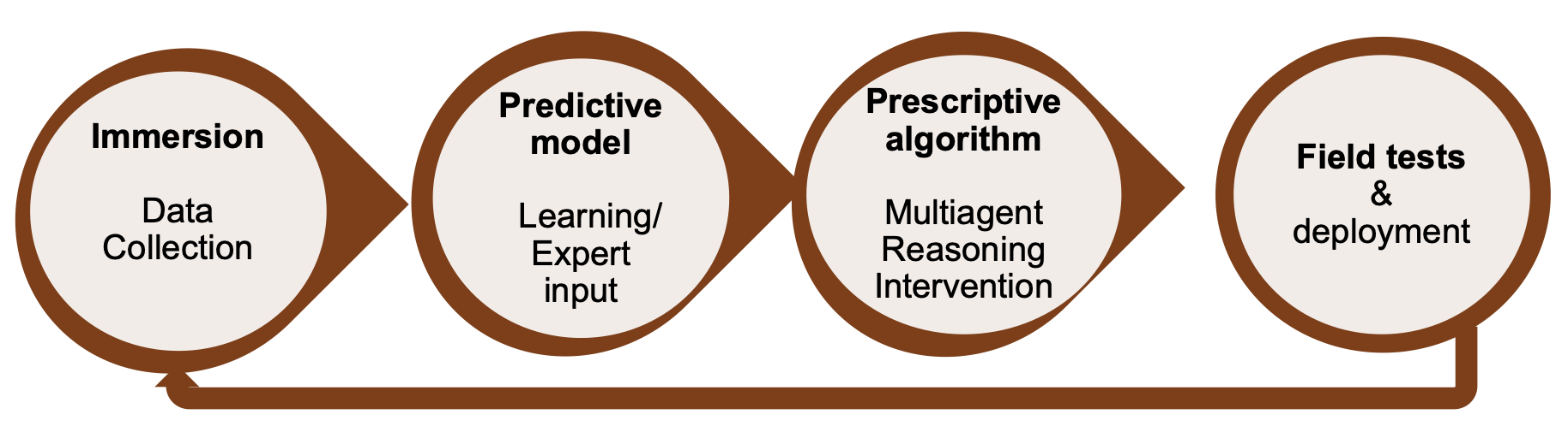
As a first step, immersion in the domain is crucial to get an understanding of the problems, constraints, and datasets. This may be a step that involves discussions with various stakeholders (including the impacted community). In this step, it is also important to build interdisciplinary partnerships and understand the challenges from the perspective of domain experts.
Following an in-depth understanding of the problem situation, the next step is building a predictive model using machine learning or domain expert input. Such a predictive model may, for example, predict high-risk vs low-risk cases in a population.
The next step is the prescriptive algorithm phase that plans interventions. Work on AI for social impact is often focused on domains where access to data is difficult (e.g., low resource communities or emerging market countries). Hence, the challenge is often to plan interventions despite that data is uncertain and sparse.
The final step is field testing and deployment. This phase helps researchers to learn about the social impact as well as key limitations of the models and algorithms (and might even lead to fundamentally new research questions). Crucial for this phase is the interdisciplinary partnerships with the respective communities for immersion and field testing.
In this section, we want to give an overview of some exemplary problems that have already been tackled by “AI for Social Impact” research. This list is by no means exhaustive - we merely decided to focus on areas of research that we find interesting from both a societal as well as technical perspective.
HIV is a serious threat to public health. Homeless youth is particularly susceptible to HIV spread because of injection drugs and unsafe sexual practices. It is therefore of major importance to raise awareness about HIV among homeless youth. To address this, various researchers have used techniques from sequential decision making and influence maximization.
Youth social workers routinely launch “peer leader” programs to inform selected participants about HIV prevention, hoping that these peer leaders will spread the information to other homeless youth. These programs are often constrained by their available resources (financial and HR) and cannot reach out to every homeless youth. It is therefore important to select the “right” set of peer leaders.
Previously, service providers have used the degree centrality measure in a social graph to determine which person is the most popular youth. This is not necessarily the best selection method (e.g. in cases where the peer leaders might be unwilling to spread information).
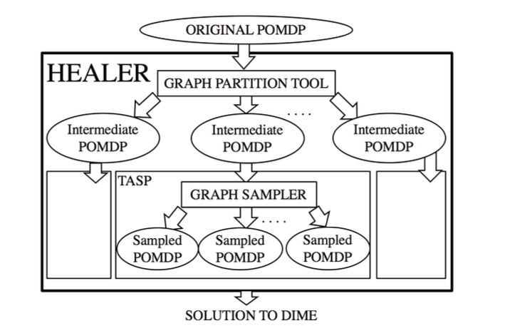
The authors formulate a planning problem in terms of a partially observable MDP (POMDP) in which they operate with the intent to maximize the influence on a social network. Since the existing POMDP solvers do not scale to the size of the problem at hand (a large “unobservable” social graph), Yadav et al. have proposed a hierarchical approach called HEALER which decomposes the POMDP into smaller ones.
HEALER then solves these smaller POMDPs using an approach called Tree Aggregation for Sequential Planning (based on a variant of the Upper Confidence Bounds algorithm applied to Trees, i.e. UCT) and subsequently aggregates the results. At each time step, the planning algorithm selects a small set of homeless youth as the “peer leader” who will participate in the program at the service provider.
The dataset in this study is the social network connectivity, i.e. which homeless youths are friends with each other. This information was gathered by parsing the youth’s Facebook contact list to determine the friendship status. The data was further augmented based on reports gathered from the service providers who perform interviews with the homeless youths.
Central to the success of the pilot study was the collaboration between the authors and homeless youth service providers. This helped to facilitate the recruitment of the youth and the implementation of the program. In addition to that, the engagement of social work researchers has also provided the necessary context and skills to communicate with the youth.
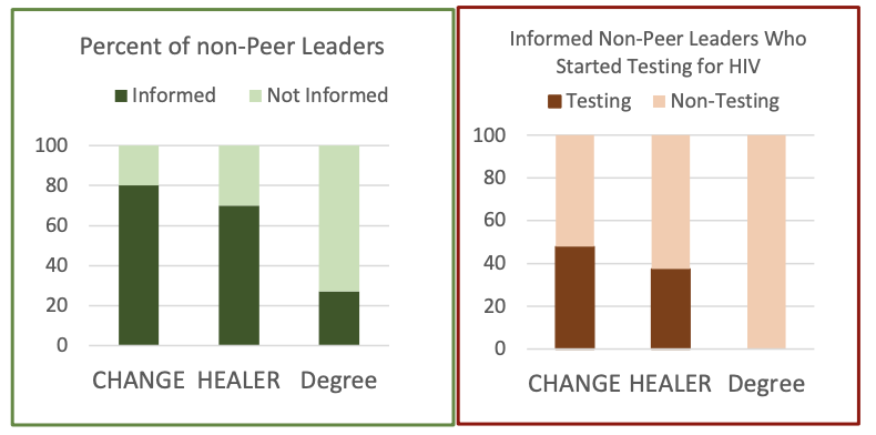
In spring 2016, the authors performed a pilot field test of HEALER, comparing it to the baseline of degree centrality. The experiment showed that HEALER is significantly more effective at spreading information - it reaches around 75% of non-peer leaders, compared to only 25% for the degree centrality approach. As a result, HEALER is more effective at causing youth to start testing for HIV: around 30-40% of the community began testing (compared to 0% for degree centrality).
Wildlife poaching is a great threat to the ecological diversity of our planet. Because of the high profits to be made from poaching, poachers have become increasingly sophisticated. Rangers protect wildlife from poachers, but to be effective, it is important to design good patrol routes for the rangers. In a series of papers, researchers have developed and deployed a suite of game-theoretic tools called “PAWS” that simulate patrol routes to combat poaching.
Patrollers in wildlife conservation areas have lots of experience conducting patrols. They design the patrol routes based on their knowledge and experience in the area. However, since the poachers are highly strategic in evading the patrollers, these patrol routes are very susceptible to gaming. While experience can help the patrollers, it may also keep the patrollers from going to underexplored areas where the poachings might be frequent. A game-theoretic planner for patrol routes can be useful in addressing these issues.
The authors propose PAWS (Protection Assistant for Wildlife Security), which is based on game-theoretic techniques usually applied in Stackelberg security games. PAWS models a two-player zero-sum game between an attacker (the poacher) and a defender (the patroller).
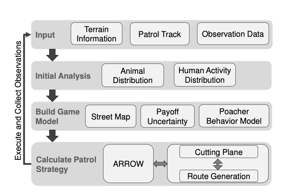
The authors use ML to learn poacher’s behavior patterns from historical data. The ML methods used have gone through several stages of development and involve (among others) a variant of decision tree ensembles, a hybrid model of decision trees and Markov random fields, as well as Gaussian Processes. Solving for the equilibrium of this game through mathematical programming gives an optimal patrol strategy for the patroller. Further enhancements to the system provide coordinated patrol plans for patrollers and use online learning to design patrols that trade-off exploitation and exploration.
PAWS uses the animal activity data to estimate the animal density which plays a role in determining the payoff of each patrol route. PAWS also uses the poacher activity data to aid the poacher modeling. All these data and previous patrol tracks are obtained from the collaborating conservation agency. To consider the terrain and elevation information, PAWS also uses topographical data.
The development of the PAWS system has been going on for several years and has involved multiple AI researchers. One of the most important factors for the successful deployment of PAWS in the wild has been the collaboration with conservation agencies. This has helped to identify suitable research problems and put the results in the field.
PAWS has been field-tested in multiple conservation sites in Uganda, Cambodia, Malaysia, and China. The authors claim that PAWS proved to be effective in all these deployments, often leading the patrollers to patrol routes never used before but discovering poacher activities on those routes. In 2019, PAWS started a partnership with SMART (a popular wildlife conservation software). This partnership will hopefully allow PAWS to be scaled to over 800 wildlife conservation sites worldwide in the near-term future.
In the global south, Community Health Workers (CHWs) play an important role in public health-care systems. CHWs complement primary health facilities by providing health education, screening, and basic emergency care in local communities. CHWs are often responsible for hundreds of patients, but only have access to limited resources (which restricts the number of patients that can be monitored and intervened each day). To maximize welfare, the CHWs’ resources need to be allocated effectively - this is commonly referred to as the health monitoring and intervention problem (HMIP).
Existing solutions to optimize HMIP do not factor risk-sensitivity into their planning models. This can entail the risk of patients being ignored as they are seen as less important to be intervened upon. In traditional HMIP models, patients are intervened upon in a round-robin order which does not consider the level of care a patient requires and might lead to more interventions than really necessary.
The authors introduce Collapsing Bandit models, a subclass of restless multi-armed bandit models (RMABs) which they claim to be able to generalize better than previous RMABs. Each bandit’s arm represents a patient, and each time an arm is played, the MAB transitions into one of the following two states:
The CHWs’ goal is to find a policy that maximizes the total reward across all arms. To find an optimal policy, the collapsing bandit model builds on the Whittle index technique and leverages Lagrangian relaxation to solve the optimization problem. As a result, the collapsing bandit model achieves a 3x-speedup compared to other RMAB techniques without impairing the model’s performance.
The experiment makes use of a real-world healthcare dataset compiled by Killian et. all. This dataset contains data from 17.000 tuberculosis patients over 292 health centers in Mumbai, India, which have received a total of 2.1 million doses and needed to follow a 6-month medication plan.
The local CHWs play an important role in building a bridge between health resources and local communities. With directly observed treatments, CHWs can observe and confirm directly that a patient is taking the prescribed medications. Despite this, the social stigma of public fear of illness and the financial burden on patients to travel to health facilities might still increase the likelihood that follow-up visits might be missed.
For this reason, digital adherence technology (DAT) plays an important role in supporting the eradication of diseases such as tuberculosis by observing the adherence to medication electronically. Patients can for example send a text message or provide a photo of their pillboxes to prove the drug intake, which allows CHWs to focus their limited time on high-risk patients.
The authors have evaluated their algorithm on a variety of datasets, including real and synthetic data. In particular, Mate et al. used tuberculosis medication adherence data from Killian et. all. To the best of the knowledge of the authors of this blog post, no RMAB-based planning framework for health intervention has been put into production yet.
Looking into the future, we believe AI is of major importance for improving society and fighting social injustice. To that end, in pushing forward the agenda of §AI for Social Impact”, we need to engage in interdisciplinary collaborations and bring the benefits of AI to populations that have not benefited from it so far.
We hope that you found the case studies that we presented useful. In publishing this blog post, we wish to demonstrate the social impact that AI can have in the real world. From our perspective, we are only at the beginning of the journey.
Further References:
Authors:
If you want to interact with the bot, you must include #FamousQuotesFromRoding
in your tweet and it’ll reply to you (Roding is a small village in Bavaria and also my hometown).
The bot works by using Markov chains, which can generate text that looks superficially good, but is actually quite nonsensical. I trained it on Adam Smith’s book “An Inquiry into the Nature and Causes of the Wealth of Nations”, so don’t be surprised if it engages with you in a discusson on free markets and economic affairs.
At some point in the future, I might consider to improve the bot to work with GPT2 (or another language model) or write up a more detailed blog post on the tech stack that I used to deploy the bot (Google Cloud App Engine).
]]>Towards the end of last year, I had the pleasure to compete in the Pacman CTF competition that was run as part of the COMP90054 course at the University of Melbourne (Semester 2 2020).
The CTF competition involves a multi-player capture-the-flag variant of Pacman in which the students make use of classical planning as well as reinforcement learning techniques to design agents that play Pacman against each other in a tournament.
The objective of the Pacman agents is to eat as much food as possible on the far side of the map, while defending the food on their home side (the contest was originally designed by Berkley and is described in further detail here).
In accordance with the COMP90054 Code of Honour, my team and I are not allowed to release the code that we used for our Pacman agents, but nonethless I would like to use this blog post to discuss which approaches we considered and which we found to perform best in the competition.
If you are interested in further details, please refer to the Wiki that is part of the following repository: COMP90054-Pacman-Competition
At the beginning of the competition, we experimented with a variety of techniques such as classical planning with PDDL or value iteration using a model-based MDP. In the interest of time (the competition took approx. 6 weeks), we decided to settle on two main approaches with which we competed in the tournament and achieved satisfying results (top 10% position in the leaderboard).
These two approaches were: 1. Approximate Q-Learning 2. Behaviour Trees with A-Star Heuristic Search
In the remainder of this blog post, I would like to talk about the various advantages and disadvantages of both techniques.
The motivation for this approach was to produce approximate Q-learning agent(s) (both offensive and defensive) which learns feature-weights of states (described below) that enable the agent to act within the Pacman contest environment.
Approximate Q-Learning is a means of approximating the Q-functions used in traditional/simple Q-learning. This method utilises reward shaping (providing an agent with useful, intermediate rewards) in addition to function approximation in order to reduce a once-exponentially large state space into a more feasible domain. This is done by:
Extracting features deemed necessary for the problem task;
Performing updates on the weights of said features;
Estimating Q-values by summing features and their weights.
The following is a list of improvements that eventually became the behaviour protocols to which we attribute the agent’s success:
The motivation for this approach was to produce an agent which uses behaviour trees as well as A* heuristic search to accomplish different goals within the Pacman contest environment.
Behaviour trees are trees containing hierarchical nodes which control the flow of decision making of agents. These trees are defined as directed acyclic graphs with internal nodes corresponding with events/stimuli, and external nodes corresponding with behaviours (in contrast with hierarchical state machines whereby stimuli leads to states, rather than behaviours). The image below illustrates a simplistic behaviour tree for a two-armed robot (By Aliekor at English Wikipedia, CC BY-SA 3.0, https://commons.wikimedia.org/w/index.php?curid=39804218):
A* (“A star”) is a heuristic search algorithm which generates a lowest-cost path tree from the start node to the goal node. A* utilises a function f(n) which provides an estimate of the total cost of a path from node n. The function f(n) is calculated as f(n) = g(n) + h(n), whereby g(n) is the cost to reach node n, and h(n) is the estimated cost from n to the goal node (requiring a heuristic cost function). A* is complete for safe heuristics and optimal for admissible heuristics.
An agent utilising a behaviour tree would be able smart and informed decisions which have been pre-programmed by the agent-designer. Possibilities for evolving behaviour would stem from manual supervision of matches in an effort to assess which stimuli should trigger certain behaviours.
Features:
Other parameters:
Features:
Additionally, the training hyper-parameters (how will the agent’s Q-function be structured? i.e. how will the agent learn? what are its priorities?), were tuned in an effort to optimise training for both agents; hyper-parameters described below:
It’s an essential read for every knowledge worker out there in the economy as it covers the constant distractions and temptations that we face (coming from an endless flow of e-mails, social media activity etc.) and provides helpful guidance on how we can structure our lifes to become more focused and more productive (in terms of getting the type of work done that really matters).
Even though I found some of the advice that he gives a little bit too intrusive for me (e.g. disconnecting from all of social media for a full 30 days straight), I can nonetheless absolutely imagine the benefits that following his advice might bring.
]]>The first blog post is a rather technical introduction to the diagnostics capabilities of modern cars, while the second blog post elaborates a bit more on what it takes to take such a product from concept stage to implementation stage.
Upon personal reflection, I think that connected car services are a highly interesting topic for future research and I’m already more than excited for the next opportunity to explore this topic further!
Post 1: OBD - a heavily underrated bridging technology for the implementation of connected car scenarios
Post 2: Leveraging OBD access to build up functional and technical capabilities for connected car services
]]>